CPPN Networks
The compositional pattern-producing network (CPPN) was invented by Stanley (2007) and is a variation of the artificial neural network. CPPN recognizes one biologically plausible fact. In nature, genotypes and phenotypes are not identical. In other words, the genotype is the DNA blueprint for an organism. The phenotype is what actually results from that plan.
In nature, the genome is the instructions for producing a phenotype that is much more complex than the genotype. In the original NEAT, as seen in the last section, the genome describes link for link and neuron for neuron how to produce the phenotype. However, CPPN is different because it creates a population of special NEAT genomes. These genomes are special in two ways. First, CPPN doesn’t have the limitations of regular NEAT, which always uses a sigmoid activation function. CPPN can use any of the following activation functions:
- Clipped linear
- Bipolar steepened sigmoid
- Gaussian
- Sine
- Others you might define
You can see these activation functions in Figure 1:
Figure 1: CPPN Activation Functions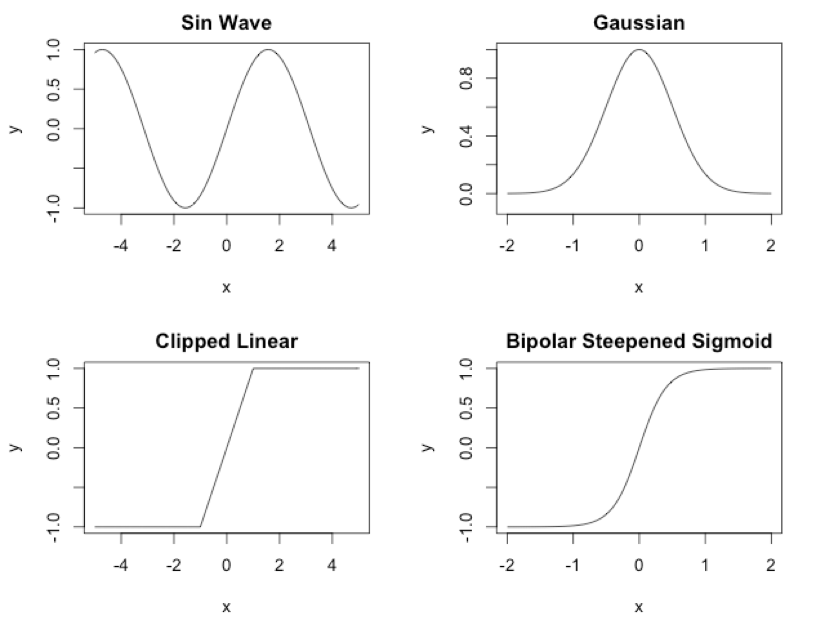
The second difference is that the NEAT networks produced by these genomes are not the final product. They are not the phenotype. However, these NEAT genomes do know how to create the final product.
The final phenotype is a regular NEAT network with a sigmoid activation function. We can use the above four activation functions only for the genomes. The ultimate phenotype always has a sigmoid activation function.
CPPN Phenotype
CPPNs are typically used in conjunction with images, as the CPPN phenotype is usually an image. Though images are the usual product of a CPPN, the only real requirement is that the CPPN compose something, thereby earning its name of compositional pattern-producing network. There are cases where a CPPN does not produce an image. The most popular non-image producing CPPN is HyperNEAT, which is discussed in the next section.
Creating a genome neural network to produce a phenotype neural network is a complex but worthwhile endeavor. Because we are dealing with a large number of input and output neurons, the training times can be considerable. However, CPPNs are scalable and can reduce the training times.
Once you have evolved a CPPN to create an image, the size of the image (the phenotype) does not matter. It can be 320x200, 640x480 or some other resolution altogether. The image phenotype, generated by the CPPN will grow to the size needed. As we will see in the next section, CPPNs give HyperNEAT the same sort of scalability.
We will now look at how a CPPN, which is itself a NEAT network, produces an image, or the final phenotype. The NEAT CPPN should have three input values: the coordinate on the horizontal axis (x), the coordinate on the vertical axis (y), and the distance of the current coordinate from the center (d). Inputting d provides a bias towards symmetry. In biological genomes, symmetry is important. The output from the CPPN corresponds to the pixel color at the x-coordinate and y-coordinate. The CPPN specification only determines how to process a grayscale image with a single output that indicates intensity. For a full-color image, you could use output neurons for red, green, and blue. Figure 2 shows a CPPN for images:
Figure 2: CPPN for Images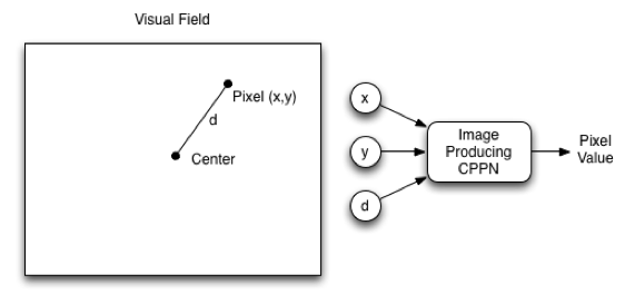
You can query the above CPPN for every x-coordinate and y-coordinate needed. Listing 1 shows the pseudocode that you can use to generate the phenotype:
Listing 1: Generate CPPN Image
1 | def render_cppn(net,bitmap): |
The above code simply loops over every pixel and queries the CPPN for the color at that location. The x-coordinate and y-coordinate are normalized to being between -1 and +1. You can see this process in action at the Picbreeder website at following URL:
Depending on the complexity of the CPPN, this process can produce images similar to Figure 2:
Figure 3: A CPPN-Produced Image (picbreeder.org)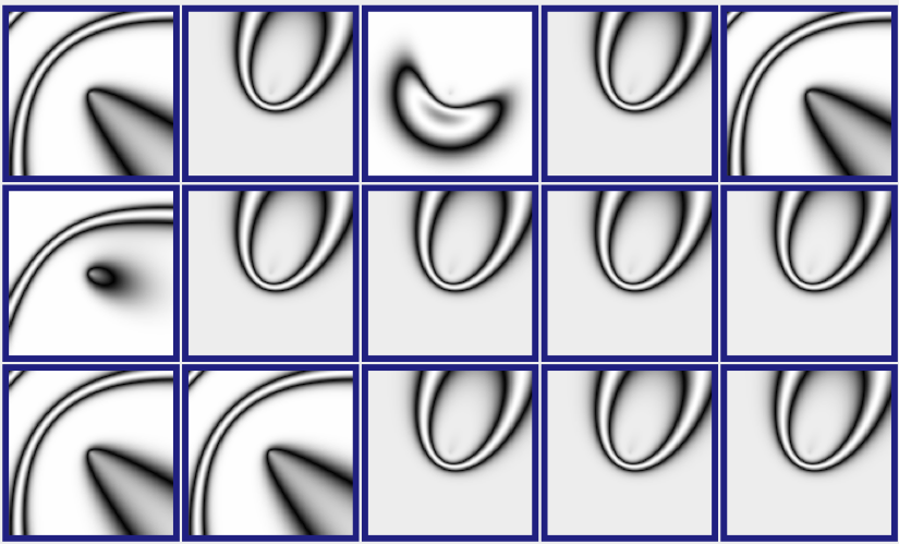
Picbreeder allows you to select one or more parents to contribute to the next generation. We selected the image that resembles a mouth, as well as the image to the right. Figure 3 shows the subsequent generation that Picbreeder produced.
Figure 3: A CPPN-Produced Image (picbreeder.org)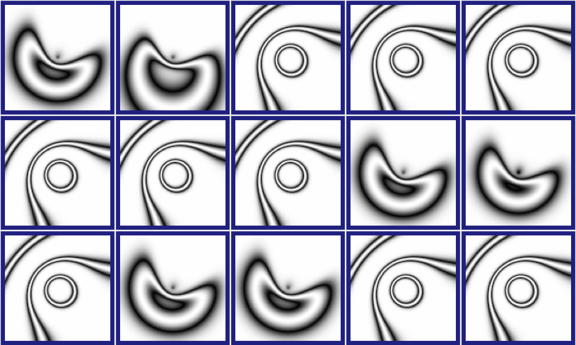
CPPN networks handle symmetry just like human bodies. With two hands, two kidneys, two feet, and other body part pairs, the human genome seems to have a hierarchy of repeated features. Instructions for creating an eye or various tissues do not exist. Fundamentally, the human genome does not have to describe every detail of an adult human being. Rather, the human genome only has to describe how to build an adult human being by generalizing many of the steps. This greatly simplifies the amount of information that is needed in a genome.
Another great feature of the image CPPN is that you can create the above images at any resolution and without retraining. Because the x–coordinate and y–coordinate are normalized to between -1 and +1, you can use any resolution.
HyperNEAT Networks
HyperNEAT networks, invented by Stanley, D’Ambrosio, & Gauci (2009), are based upon the CPPN; however, instead of producing an image, a HyperNEAT network creates another neural network. Just like the CPPN in the last section, HyperNEAT can easily create much higher resolution neural networks without retraining.
HyperNEAT Substrate
One interesting hyper-parameter of the HyperNEAT network is the substrate that defines the structure of a HyperNEAT network. A substrate defines the x-coordinate and the y-coordinate for the input and output neurons. Standard HyperNEAT networks usually employ two planes to implement the substrate. Figure 4 shows the sandwich substrate, one of the most common substrates:
Figure 4: HyperNEAT Sandwich Substrate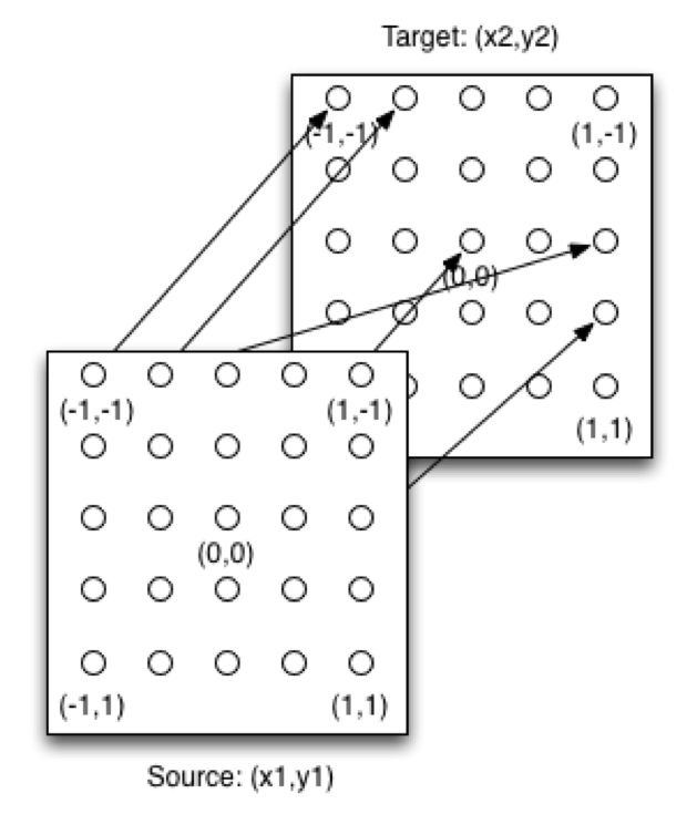
Together with the above substrate, a HyperNEAT CPPN is capable of creating the phenotype neural network. The source plane contains the input neurons, and the target plane contains the output neurons. The x-coordinate and the y-coordinate for each are in the -1 to +1 range. There can potentially be a weight between each of the source neurons and every target neuron. Figure 8.8 shows how to query the CPPN to determine these weights:
Figure 5: Sandwich Substrate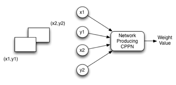
The input to the CPPN consists of four values: x1, y1, x2, and y2. The first two values x1 and y1 specify the input neuron on the source plane. The second two values x2 and y2 specify the input neuron on the target plane. HyperNEAT allows the presence of as many different input and output neurons as desired, without retraining. Just like the CPPN image could map more and more pixels between -1 and +1, so too can HyperNEAT pack in more input and output neurons.
HyperNEAT Computer Vision
Computer vision is a great application of HyperNEAT, as demonstrated by the rectangles experiment provided in the original HyperNEAT paper by Stanley, Kenneth O., et al. (2009). This experiment placed two rectangles in a computer’s vision field. Of these two rectangles, one is always larger than the other. The neural network is trained to place a red rectangle near the center of the larger rectangle. Figure 8.9 shows this experiment running under the Encog framework:
Figure 8.9: Boxes Experiment (11 resolution)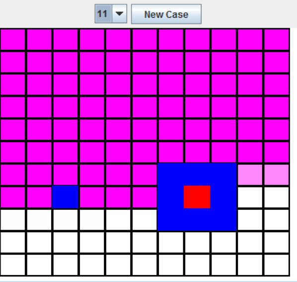
As you can see from the above image, the red rectangle is placed directly inside of the larger of the two rectangles. The “New Case” button can be pressed to move the rectangles, and the program correctly finds the larger rectangle. While this works quite well at 11x11, the size can be increased to 33x33. With the larger size, no retraining is needed, as shown in Figure 6:
Figure 6: Boxes Experiment (33 resolution)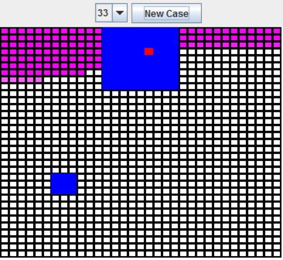
When the dimensions are increased to 33x33, the neural network is still able to place the red square inside of the larger rectangle.
The above example uses a sandwich substrate with the input and output plane both equal to the size of the visual field, in this case 33x33. The input plane provides the visual field. The neuron in the output plane with the highest output is the program’s guess at the center of the larger rectangle.