The goal of this article is to help you understand what a neural network is, and how it is used. Most people, even non-programmers, have heard of neural networks. There are many science fiction overtones associated with them. And like many things, sci-fi writers have created a vast, but somewhat inaccurate, public idea of what a neural network is.
Most laypeople think of neural networks as a sort of artificial brain. Neural networks would be used to power robots or carry on intelligent conversations with human beings. This notion is a closer definition of Artificial Intelligence (AI), than neural networks. AI seeks to create truly intelligent machines. I am not going to waste several paragraphs explaining what true, human intelligence is, compared to the current state of computers. Anyone who has spent any time with both human beings and computers knows the difference. Current computers are not intelligent.
Neural networks are one small part of AI. Neural networks, at least as they currently exist, carry out very small specific tasks. Computer based neural networks are not a general-purpose computation device, like the human brain. Perhaps some of the confusion comes from the fact that the brain itself is a network of neurons, or a neural network. This brings up an important distinction.
The human brain really should be called a biological neural network (BNN). This article is not about biological neural networks. This article is about artificial neural networks (ANN). Most texts do not bother to make the distinction between the two. This article is the same. When I refer to a neural network, I actually mean an artificial neural network.
There are some basic similarities between biological neural networks and artificial neural networks. But they are very basic similarities. Artificial neural networks are largely mathematical constructs that were inspired by biological neural networks. An important term that is often used to describe various artificial neural network algorithms is biological plausibility. This term defines how close an artificial neural network algorithm is to a biological neural network.
Like I said, neural networks are designed to accomplish one small task. A full application will likely use neural networks to accomplish certain parts of the application. The entire application will not be implemented as a neural network. The application may be made of several neural networks, each designed for a specific task.
The task that neural networks accomplish very well is pattern recognition. You communicate a pattern to a neural network and it communicates a pattern back to you. At the highest level, this is all that a typical neural network does. Some network architectures will vary this, but the vast majority of neural networks in place work this way. Figure 1 illustrates a neural network at this level.

Figure 1: A Typical Neural Network
As you can see, the neural network above is accepting a pattern and returning a pattern. Neural networks operate completely synchronously. A neural network will only output when presented with input. It is not like a human brain, which does not operate exactly synchronously. The human brain responds to input, but it will produce output anytime it feels like it!
Neural Network Structure
Neural networks are made of layers of similar neurons. Most neural networks have at least an input layer and output layer. The input pattern is presented to the input layer. Then the output pattern is returned from the output layer. What happens between the input and output layers is a black box. At this point in the article, we are not yet concerned with the internal structure of the neural network. There are many different architectures that define what happens between the input and output layer. Later in this article, we will examine some of these architectures.
The input and output patterns are both arrays of floating point numbers. You could think of it as follows.
1 | Neural Network Input: [ -0.245, .283, 0.0 ] |
The neural network above has three neurons in the input layer, and two neurons in the output layer. The number of neurons in the input and output layers do not change. As a result, the number of elements in the input and output patterns, for a particular neural network, can never change.
To make use of the neural network you must express your problem in such a way as to have the input to the problem be an array of floating point numbers. Likewise, the solution to the problem must be an array of floating point numbers. This is really all that neural networks can do for you. They take one array and transform it into a second. Neural networks do not loop, call subroutines, or perform any of the other tasks you might think of with traditional programming. Neural networks recognize patterns.
You might think of a neural network as something like a hash table in traditional programming. In traditional programming, a hash table is use to map keys to values. Somewhat like a dictionary. The following could be thought up as a hash table.
1 | "hear" -> "to perceive or apprehend by the ear" |
This is a mapping between words and the definition of each word. This is a hash table, just as you might see in any programming language. It uses a key of string, to another value of a string. You provide the dictionary with a key, it returns a value. This is how most neural networks function. One neural network called a BAM, or bidirectional associative memory actually allows you to also pass in the value and receive the key.
Programming hash tables use keys and values. Think of the pattern sent to the input layer of the neural network as they key to the hash table. Likewise, think of the value returned from the hash table as the pattern that is returned from the output layer of the neural network. The comparison between a hash table and a neural network works well; however, the neural network is much more than a hash table.
What would happen, with the above hash table, if you were to pass in a word that is not a key in the map? For example, if you were to pass in the key of ìwroteî. A hash table would return null, or in some way indicate that it could not find the specified key. Neural networks do not return null! They find the closest match. Not only do they find the closest math, they will modify the output to guess at what it would be for the missing value. So if you passed ìwroteî to the neural network above, you would likely get back what you would have expected for ìwriteî. There is not enough data for the neural network to have modified the response, as there are only three samples. So you would likely get the output from one of the other keys.
The above mapping brings up one very important point about neural networks. Recall, I said that neural networks accept an array of floating point numbers, and return another array? How would you put strings into the neural network, as seen above? There is a way to do this, but generally, it is much easier to deal with numeric data than strings. However, we will cover how to pass strings to neural networks later in this article.
This is one of the most difficult aspects of neural network programming. How do you translate your problem into a fixed-length array of floating point numbers? This is the aspect of neural network programming that is often the most difficult to ìget your head aroundî. The best way to demonstrate this is with several examples.
A Simple Example
If you have read anything about neural networks you have no doubt seen examples with the XOR operator. The XOR operator is essentially the ìHello Worldî of neural network programming. This article will describe scenarios much more complex than XOR. The XOR operator is a great introduction. We shall begin by looking at the XOR operator as though it were a hash table. If you are not familiar with the XOR operator, it works similar to the AND and OR operators. For an AND to be true, both sides must be true. For an OR to be true, either side must be true. For an XOR to be true, both of the sides must be different from each other. The truth table for an XOR is as follows.
1 | False XOR False = False |
To continue the hash table example, the above truth table would be represented as follows.
1 | [ 0.0 , 0.0 ] -> [ 0.0 ] |
These mapping show input, and the ideal expected output for the neural network.
Training: Supervised and Unsupervised
When you specify the ideal output you are using something called supervised training. If you did not provide ideal outputs, you would be using unsupervised training.
Supervised training teaches the neural network to produce the ideal output. Unsupervised training usually teaches the neural network to group the input data into a number of groups defined by the output neuron count.
Both supervised and unsupervised training is an iterative process. For supervised training, each training iteration calculates how close the actual output is to the ideal output. This closeness is expressed as an error percent. Each iteration modifies the internal weight matrixes of the neural network to get the error rate to a low enough level.
Unsupervised training is also an iterative process. Calculating the error is not quite as easy, however. You have no expected output, so you cannot measure how far the unsupervised neural network is from your ideal output, you have no ideal output. Often you will just iterate for a fixed number of iterations and then try to use the network. If it needs more training, then that training is provided.
Another very important aspect to the above training data is that it can be taken in any order. The result of 0 XOR 0 is going to be 0, regardless of which case you just looked at. This is not true of all neural networks. For the XOR operator we would probably use a neural network type called a feedforward perceptron. Order does not matter to a feedforward neural network. Later in this chapter we will see a simple recurrent neural network. Order becomes very important for a simple recurrent neural network.
You saw how training data was used for the simple XOR operator. Now we will look at a slightly more complex scenario.
Miles per Gallon
Usually neural network problems involve dealing with a set of statistics. You will try to use some of the statistics to predict the others. Consider a car database. It contains the following fields.
1 | Car weight |
I am somewhat oversimplifying the data, but this is more to show how to format data. Assuming you have collected some data for these fields, you should be able to construct a neural network that can predict one field value, based on the other field values. For this example, we will try to predict miles-per-gallon.
Recall, from before, that we will need to define this problem in terms of an input array of floating points mapped to an output array of floating points. However, there is one additional requirement. The numeric range on each of these array elements should be between 0 and 1 or -1 and 1. This is called normalization. Taking real-world data and turning it into a form that the neural network can process.
First we see how we would normalize data from above. First, consider the neural network format. We have six total fields. We want to use five of these to predict the sixth. The neural network would have five input neurons and one output neuron.
Your network would look something like the following.
1 | Input Neuron 1: Car weight |
We also need to normalize the data. To do this we must think of reasonable ranges for each of these values. We will then transform input data into a number between 0 and 1 that represents an actual value”s position within that range. We will now look at an example. We will establish reasonable ranges for these values as follows.
1 | Car weight: 100-5000 lbs |
These ranges may be a little large, given today’s cars. However, this will allow minimal restructuring to the neural network in the future. It is also good to not have too much data at the extreme ends of the range.
We will now look at an example. How would we normalize a weight of 2,000 pounds? This weight is 1,900 into the range (2000 - 100). The size of the range is 4,900 pounds (5000-100). The percent of the range size is 0.38 (1,900 / 4,900). Therefore we would feed the value of 0.38 to the input neuron to represent this value. This satisfies the range requirement of 0 to 1 for an input neuron.
The hybrid or regular value is a true/false. To represent this value we will use a 1 for hybrid and a 0 for regular. We simply normalize a true/false into two values.
Presenting Images to Neural Networks
Images are a popular source of input for neural networks. In this section, we will see how to normalize an image. There are more advanced methods than this, but this method is often effective.
Consider an image that might be 300x300 pixels. Additionally, the image is full color. We would have 90,000 pixels times the three RGB colors, giving 270,000 total pixels. If we had an input neuron for each pixel, that would also be 270,000 input neurons. This is just too large for an artificial neural network.
We need to downsample. Consider the following image. It is at full resolution.

We will now downsample it to 32x32.

Do you notice the grid-like pattern? It has been reduced to 32x32 pixels. These pixels would form the input to a neural network. This neural network would require 1,024 input neurons, if the network were to only look at the intensity of each square. Looking at the intensity only causes the neural network to see in ìblack and whiteî.
If you would like the neural network to see in color, then it is necessary to provide red, green and blue (RGB) values for each of these pixels. This would mean three input neurons for each pixel, which would push our input neuron count to 3,072.
These intensities are between 0 and 255, as 0 to 255 is the normal range for RGB values. Simply divide the intensity by 255 and you will be given a value the neural network can take. For example, intensity number 10 becomes 10/255, or 0.039.
You may be wondering how the output neurons will be handled. In a case such as this you would like the output neurons to communicate what image the neural network believes it is looking at. The usual solution is to create one output neuron for each type of image the neural network should recognize. The network will be trained to return a value of 1.0 for the output neuron that corresponds to what the image is believed to be.
We will continue showing you how to format neural networks for real-world problems in the next section. The next section will take a look at financial neural networks.
Financial Neural Networks
Financial neural networks are very popular form of temporal neural network. A temporal neural network is one that accepts input for values that range over time. There are two common ways that temporal data is presented to a neural network. The original method is to use an input window and a prediction window. Consider if you would like the neural network to predict the stock market. You have the following stock price information that represents the closing price for a stock over several days.
1 | Day 1: $45 |
The first step is to normalize the data. To do this we want to change each number into the percent movement from the previous day. For example, day 2 would become 0.04 percent, because $45 to $47 was a 4% move from $45. We do this with every day’s value.
1 | Day 2: 0.04 |
We would like to create a neural network that will predict the next day’s values. We need to think about how to encode this data to be presented to the neural network. The way we do this depends on if the neural network is recurrent or not. Recall from earlier in the article that I said we would treat the neural network as a black box. I said that there were hidden layers, between the input and output layers. We will now see what these layers are for. They become important now, because they will dictate the structure of the neural network.
The feedforward perceptron is a very popular neural network architecture. This neural network has one or more hidden layers. This is the type of neural network that we used for the XOR example earlier in this article. To use this network to predict stock prices we must use ìtime windowsî. We are going to use a window of three prices to predict the fourth. So to predict tomorrow we look at the previous three days. This means we will have an input layer with three neurons and an output layer with a single layer. We will feed in three days and request a prediction for the fourth. This neural network looks like Figure 2.
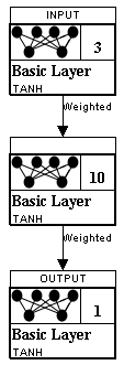
Figure 2: Feedforward Neural Network
A Feedforward Neural Network
In the above figure, you see the input and output layers. There is also a hidden layer, with ten neurons. Hidden layers help the neural network to recognize more patterns. Choosing the size of the hidden layers can be difficult. This is a topic that will be covered in future articles.
We will need to create training data for this neural network. The training data is nothing more than three days of price change information followed by an ideal value of what the next day is. You can see the training data here.
1 | [0.04, 0.02, -0.16] -> [0.02] |
Just as was the case with the XOR data, the order of the training data is not important. We are simply providing three days worth of price change for the neural network to use to predict the following day.
We will also look at how we would present this data to a simple recurrent neural network. There are several different types of simple recurrent neural network. The type we will use for this example is called an Elman neural network. For the Elman neural network we will have a single input neuron and a single output neuron. We will provide just a single day’s worth of price information and expect the next day’s price change back. Figure 3 shows an Elman neural network.
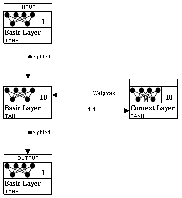
Figure 3: An Elman Neural Network
An Elman Neural Network
As you can see, the Elman neural network also has 10 hidden neurons. Just as was the case with the feedforward network, the value 10 was chosen arbitrarily. You will also notice a context layer. This context layer is recurrent; it is connected back into the neural network. The context layer allows the neural network to remember some degree of state. This will cause the output of the neural network to be dependent on more than just the last input.
Because there is a single input and output neuron, the training data is arranged differently. The training data for the Elman neural network is as follows.
1 | [0.04] -> [0.02] |
As you can see from the above data the order is very important. The neural network cannot predict tomorrow’s price seeing only today’s price. Rather, because of the context layer, the last few days will influence the output. This is very similar to the human brain. To identify a song, you will need to hear several notes in a sequence. Obviously, the order of the notes is very important.
Feeding Text to a Neural Network
Earlier I said that feeding text into a neural network is particularly challenging. You have two major issues to contend with. First, the individual words are of varying lengths. Neural networks require a fixed input and output size. Secondly, how to encode the letters can be an issue. Should the letters “A” - “Z” be stored in a single neuron, or 26 neurons, or some other way all together?
Using a recurrent neural network, such as a Elman neural network, solves part of this problem. In the last section that we did not need an input window size with the Elman neural network. We just took the stock prices one at a time. This is a great way to process letters. We will create an Elman neural network that has just enough input neurons to recognize the Latin letters and it will use a context layer to remember the ordering. Just as stock prediction uses one long stream of price changes, text processing will use one long stream of letters.
The Bag of Words algorithm is a common means of encoding strings. Each input represents the count of one particular word. The entire input vector would contain one value for each unique word. Consider the following strings.
1 | Of Mice and Men |
We have the following unique words. This is our “dictionary.”
1 | Input 0: and |
The four lines above would be encoded as follows.
1 | Of Mice and Men [0 4 5 7] |
Of course we have to fill in the missing words with zero, so we end up with the following.
1 | Of Mice and Men [1, 0, 0, 0, 1, 1, 0, 1, 0] |
Notice that we now have a consistent vector length of nine. Nine is the total number of words in our “dictionary”. Each component number in the vector is an index into our dictionary of available words. At each vector component is stored a count of the number of words for that dictionary entry. Each string will usually contain only a small subset of the dictionary. As a result, most of the vector values will be zero.
As you can see, one of the most difficult aspects of machine learning pro- gramming is translating your problem into a fixed-length array of floating point numbers. The following section shows how to translate several examples.
Conclusion
My goal in this article was to show you what a neural network is, and how you might adapt one to your application. Not every application will benefit from a neural network. In fact, most applications will not benefit from a neural network. However, for the right application a neural network can be an ideal solution. Now that you understand the fundamentals of a neural network, you are ready to take the next step and learn to program a neural network. Other resources you might find useful: