Heaton Research

Overview of Keras/TensorFlow Basic Operations

I in the process of updating my deep learning course and books to make use of Keras. This posting contains some of the basic examples that I put together. This post is not meant to be an introduction to neural networks in general. For such an introduction, refer to either my books or this article.

I will expand on these examples greatly for both the book and course. The basic neural network operations that I needed were:

  • Simple Regression
  • Regression Early Stopping
  • Simple Classification
  • Classification Early Stopping
  • Deep Neural Networks w/Dropout and Other Regularization
  • Convolutional Neural Networks
  • LSTM Neural Networks
  • Loading/Saving Neural Networks

These are some of the most basic operations that I need to perform when working with a new neural network package. This provides me with a sort of Rosetta Stone for a new neural network package. Once I have these operations, I can more easily create additional examples that are more complex.

The first thing to check is what versions you have of the required packages:

1
2
3
4
5
6
7
8
9
10
11
12
import keras
import tensorflow as tf
import sys
import sklearn as sk
import pandas as pd

print("Tensor Flow Version: {}".format(tf.__version__))
print("Keras Version: {}".format(keras.__version__))
print()
print("Python {}".format(sys.version))
print('Pandas {}'.format(pd.__version__))
print('Scikit-Learn {}'.format(sk.__version__))
1
2
3
4
5
6
Tensor Flow Version: 1.0.0
Keras Version: 2.0.6

Python 3.5.2 |Continuum Analytics, Inc.| (default, Jul 5 2016, 11:41:13) [MSC v.1900 64 bit (AMD64)]
Pandas 0.19.2
Scikit-Learn 0.18.1

The following functions are from my set of helpful functions that I created for my class and use in many of my books:

1
2
3
4
5
6
7
8
9
10
11
12
13
14
15
16
17
18
19
20
21
22
23
24
25
26
27
28
29
30
31
32
33
34
35
36
37
38
39
40
41
42
import pandas as pd
from sklearn import preprocessing

# Encode text values to dummy variables(i.e. [1,0,0],[0,1,0],[0,0,1] for red,green,blue)
def encode_text_dummy(df, name):
dummies = pd.get_dummies(df[name])
for x in dummies.columns:
dummy_name = "{}-{}".format(name, x)
df[dummy_name] = dummies[x]
df.drop(name, axis=1, inplace=True)

# Encode text values to indexes(i.e. [1],[2],[3] for red,green,blue).
def encode_text_index(df, name):
le = preprocessing.LabelEncoder()
df[name] = le.fit_transform(df[name])
return le.classes_

# Convert all missing values in the specified column to the median
def missing_median(df, name):
med = df[name].median()
df[name] = df[name].fillna(med)

# Convert a Pandas dataframe to the x,y inputs that TensorFlow needs
def to_xy(df, target):
result = []
for x in df.columns:
if x != target:
result.append(x)

# find out the type of the target column. Is it really this hard? :(
target_type = df[target].dtypes
target_type = target_type[0] if hasattr(target_type, '__iter__') else target_type

# Encode to int for classification, float otherwise. TensorFlow likes 32 bits.
if target_type in (np.int64, np.int32):
# Classification
dummies = pd.get_dummies(df[target])
return df.as_matrix(result).astype(np.float32), dummies.as_matrix().astype(np.float32)
else:
# Regression
return df.as_matrix(result).astype(np.float32), df.as_matrix([target]).astype(np.float32)

Simple Regression

Regression is where a neural network accepts several values (predictors) and produces a prediction that is numeric. In this simple example we attempt to predict the miles per gallon (MPG) of several cars based on characteristics of those cars. Several parameters and used below and described here.

  • Losses Supported by Keras
    • Typically use mean_squared_error for regression (the square root of mean square error is root mean square error(RMSE)).
    • and for classification use: binary_crossentropy for 2 classes, categorical_crossentropy for more than 2 classes.
  • kernel_initializer supported by Keras - Species how the weights of are randomized.
  • activation - Usually relu or softmax will be used.
1
2
3
4
5
6
7
8
9
10
11
12
13
14
15
16
17
18
19
20
21
22
from keras.models import Sequential
from keras.layers.core import Dense, Activation
import pandas as pd
import io
import requests
import numpy as np
from sklearn import metrics

url="https://raw.githubusercontent.com/jeffheaton/t81_558_deep_learning/master/data/auto-mpg.csv"
df=pd.read_csv(io.StringIO(requests.get(url).content.decode('utf-8')),na_values=['NA','?'])

cars = df['name']
df.drop('name',1,inplace=True)
missing_median(df, 'horsepower')
x,y = to_xy(df,"mpg")

model = Sequential()
model.add(Dense(10, input_dim=x.shape[1], activation='relu'))
model.add(Dense(1, kernel_initializer='normal'))
model.compile(loss='mean_squared_error', optimizer='adam')

model.fit(x,y,verbose=2,epochs=100)
1
2
3
4
5
6
7
8
9
10
11
12
13
14
15
16
17
18
Epoch 1/100
0s - loss: 2240.8034
Epoch 2/100
0s - loss: 1469.8520
Epoch 3/100
0s - loss: 1038.2052
Epoch 4/100
0s - loss: 820.4976
Epoch 5/100

...

0s - loss: 560.3524
Epoch 99/100
0s - loss: 559.7951
Epoch 100/100
0s - loss: 559.2341
<keras.callbacks.History at 0x2263d8cc518>

Now that the neural network is trained, we will test how good it is and perform some sample predictions.

1
2
3
4
5
6
7
8
9
pred = model.predict(x)

# Measure RMSE error. RMSE is common for regression.
score = np.sqrt(metrics.mean_squared_error(pred,y))
print("Final score (RMSE): {}".format(score))

# Sample predictions
for i in range(10):
print("{}. Car name: {}, MPG: {}, predicted MPG: {}".format(i+1,cars[i],y[i],pred[i]))
1
2
3
4
5
6
7
8
9
10
11
Final score (RMSE): 3.494112253189087
1. Car name: chevrolet chevelle malibu, MPG: [ 18.], predicted MPG: [ 14.94231319]
2. Car name: buick skylark 320, MPG: [ 15.], predicted MPG: [ 14.08107567]
3. Car name: plymouth satellite, MPG: [ 18.], predicted MPG: [ 15.15124226]
4. Car name: amc rebel sst, MPG: [ 16.], predicted MPG: [ 15.84413433]
5. Car name: ford torino, MPG: [ 17.], predicted MPG: [ 15.11468124]
6. Car name: ford galaxie 500, MPG: [ 15.], predicted MPG: [ 10.48310184]
7. Car name: chevrolet impala, MPG: [ 14.], predicted MPG: [ 10.11642265]
8. Car name: plymouth fury iii, MPG: [ 14.], predicted MPG: [ 10.33946323]
9. Car name: pontiac catalina, MPG: [ 14.], predicted MPG: [ 10.317276]
10. Car name: amc ambassador dpl, MPG: [ 15.], predicted MPG: [ 12.37194347]

Regression (Early Stop)

Early stopping sets aside a part of the data to be used to validate the neural
network. The neural network is trained with the training data and validated
with the validation data. Once the error no longer improves on the validation
set, the training stops. This prevents the neural network from overfitting.

1
2
3
4
5
6
7
8
9
10
11
12
13
14
15
16
17
18
19
20
21
22
23
24
25
26
27
28
29
import pandas as pd
import io
import requests
import numpy as np
from sklearn import metrics
from keras.models import Sequential
from keras.layers.core import Dense, Activation
from keras.callbacks import EarlyStopping

url="https://raw.githubusercontent.com/jeffheaton/t81_558_deep_learning/master/data/auto-mpg.csv"
df=pd.read_csv(io.StringIO(requests.get(url).content.decode('utf-8')),na_values=['NA','?'])

cars = df['name']
df.drop('name',1,inplace=True)
missing_median(df, 'horsepower')
x,y = to_xy(df,"mpg")

# Split into train/test
x_train, x_test, y_train, y_test = train_test_split(
x, y, test_size=0.25, random_state=45)

model = Sequential()
model.add(Dense(10, input_dim=x.shape[1], kernel_initializer='normal', activation='relu'))
model.add(Dense(1, kernel_initializer='normal'))
model.compile(loss='mean_squared_error', optimizer='adam')

monitor = EarlyStopping(monitor='val_loss', min_delta=1e-3, patience=5, verbose=1, mode='auto')

model.fit(x,y,validation_data=(x_test,y_test),callbacks=[monitor],verbose=2,epochs=1000)
1
2
3
4
5
6
7
8
9
10
11
12
13
14
15
16
17
18
19
20
21
22
23
Train on 398 samples, validate on 100 samples
Epoch 1/1000
0s - loss: 374.7638 - val_loss: 179.2396
Epoch 2/1000
0s - loss: 199.9990 - val_loss: 169.4834
Epoch 3/1000
0s - loss: 197.9431 - val_loss: 153.8338
Epoch 4/1000
0s - loss: 187.7644 - val_loss: 152.2758
Epoch 5/1000
0s - loss: 185.5505 - val_loss: 149.9817

...

Epoch 179/1000
0s - loss: 10.3191 - val_loss: 8.2763
Epoch 180/1000
0s - loss: 10.0629 - val_loss: 8.3435
Epoch 181/1000
0s - loss: 10.7124 - val_loss: 8.4712
Epoch 182/1000
0s - loss: 10.6406 - val_loss: 8.4272
<keras.callbacks.History at 0x222a8ecd1d0>

Classification Model (Early Stop)

Early stopping can also be used with classification. Early stopping sets aside a part of the data to be used to validate the neural network. The neural network is trained with the training data and validated with the validation data. Once the error no longer improves on the validation set, the training stops. This prevents the neural network from overfitting.

1
2
3
4
5
6
7
8
9
10
11
12
13
14
15
16
17
18
19
20
21
22
23
24
25
26
27
28
import pandas as pd
import io
import requests
import numpy as np
from sklearn import metrics
from keras.models import Sequential
from keras.layers.core import Dense, Activation
from keras.callbacks import EarlyStopping

url="https://raw.githubusercontent.com/jeffheaton/t81_558_deep_learning/master/data/iris.csv"
df=pd.read_csv(io.StringIO(requests.get(url).content.decode('utf-8')),na_values=['NA','?'])

species = encode_text_index(df,"species")
x,y = to_xy(df,"species")

# Split into train/test
x_train, x_test, y_train, y_test = train_test_split(
x, y, test_size=0.25, random_state=45)

model = Sequential()
model.add(Dense(10, input_dim=x.shape[1], kernel_initializer='normal', activation='relu'))
model.add(Dense(1, kernel_initializer='normal'))
model.add(Dense(y.shape[1],activation='softmax'))
model.compile(loss='categorical_crossentropy', optimizer='adam')

monitor = EarlyStopping(monitor='val_loss', min_delta=1e-3, patience=5, verbose=1, mode='auto')

model.fit(x,y,validation_data=(x_test,y_test),callbacks=[monitor],verbose=2,epochs=1000)
1
2
3
4
5
6
7
8
9
10
11
12
13
14
15
16
17
18
19
20
Train on 150 samples, validate on 38 samples
Epoch 1/1000
0s - loss: 1.1095 - val_loss: 1.1143
Epoch 2/1000
0s - loss: 1.1065 - val_loss: 1.1096
Epoch 3/1000
0s - loss: 1.1041 - val_loss: 1.1057
Epoch 4/1000
0s - loss: 1.1020 - val_loss: 1.1038
Epoch 5/1000
0s - loss: 1.1011 - val_loss: 1.1017

...

Epoch 325/1000
0s - loss: 0.1758 - val_loss: 0.1320
Epoch 326/1000
0s - loss: 0.1755 - val_loss: 0.1332
Epoch 00325: early stopping
<keras.callbacks.History at 0x222a9242d68>

Show the predictions (raw, probability of each class.)

1
2
3
4
5
6
# Print out the raw predictions. Because there are 3 species of iris, there are 3 columns.  The number in each column is
# the probability that the flower is that type of iris.

np.set_printoptions(suppress=True)
pred = model.predict(x_test)
print(pred[0:10])
1
2
3
4
5
6
7
8
9
10
[[ 0.97540218  0.0245978   0.        ]
[ 0.94149685 0.05850318 0. ]
[ 0.02133332 0.27963796 0.69902873]
[ 0.94382465 0.05617536 0. ]
[ 0.95254719 0.04745276 0. ]
[ 0.95966363 0.04033642 0. ]
[ 0.94291645 0.05708356 0. ]
[ 0.00293462 0.06093681 0.93612856]
[ 0.00873046 0.14257514 0.84869444]
[ 0.00293431 0.0609317 0.93613404]]
1
2
3
4
5
# The to_xy function represented the input in the same way.  Each row has only 1.0 value because each row is only one type
# of iris. This is the training data, we KNOW what type of iris it is. This is called one-hot encoding. Only one value
# is 1.0 (hot)

print(y_test[0:10])
1
2
3
4
5
6
7
8
9
10
[[ 1.  0.  0.]
[ 1. 0. 0.]
[ 0. 0. 1.]
[ 1. 0. 0.]
[ 1. 0. 0.]
[ 1. 0. 0.]
[ 1. 0. 0.]
[ 0. 0. 1.]
[ 0. 0. 1.]
[ 0. 0. 1.]]
1
2
3
4
5
6
7
from sklearn.metrics import log_loss

# Using the predictions (pred) and the known 1-hot encodings (y_test) we can compute the log-loss error.
# The lower a log loss the better. The probabilities (pred) from the previous section specify how sure the neural network
# is of its prediction. Log loss error pubishes the neural network (with a lower score) for very confident, but wrong,
# classifications.
print(log_loss(y_test,pred))
1
0.133210815783
1
2
3
4
5
6
7
8
9
# Usually the column (pred) with the highest prediction is considered to be the prediction of the neural network.  It is easy
# to convert the predictions to the expected iris species. The argmax function finds the index of the maximum prediction
# for each row.

predict_classes = np.argmax(pred,axis=1)
expected_classes = np.argmax(y_test,axis=1)

print("Predictions: {}".format(predict_classes))
print("Expected: {}".format(expected_classes))
1
2
3
4
5
6

Predictions: [0 0 2 0 0 0 0 2 2 2 0 2 2 2 2 0 2 2 0 1 1 1 2 1 0 2 1 1 0 1 1 1 2 2 0 2 0
0]
Expected: [0 0 2 0 0 0 0 2 2 2 0 2 2 2 2 0 2 2 0 1 1 1 2 1 0 2 1 1 0 1 1 1 2 2 0 2 0
0]

1
2
3
# Of course it is very easy to turn these indexes back into iris species.  We just use the species list that we created earlier.

print(species[predict_classes[1:10]])
1
2
['Iris-setosa' 'Iris-virginica' 'Iris-setosa' 'Iris-setosa' 'Iris-setosa'
'Iris-setosa' 'Iris-virginica' 'Iris-virginica' 'Iris-virginica']
1
2
3
4
5
6
7
from sklearn.metrics import accuracy_score

# Accuracy might be a more easily understood error metric. It is essentially a test score. For all of the iris predictions,
# what percent were correct? The downside is it does not consider how confident the neural network was in each prediction.

correct = accuracy_score(expected_classes,predict_classes)
print("Accuracy: {}".format(correct))
1
Accuracy: 1.0

Deeper Networks

Keras makes it easy to add addition layers as shown here:

1
2
3
4
5
6
7
8
9
10
11
12
13
14
15
16
17
18
19
20
21
22
23
24
25
26
27
28
29
30
31
32
33
34
35
36
37
38
39
40
import pandas as pd
import io
import requests
import numpy as np
from sklearn import metrics
from keras.callbacks import EarlyStopping
from keras.layers import Dense, Dropout
from keras import regularizers

url="https://raw.githubusercontent.com/jeffheaton/t81_558_deep_learning/master/data/auto-mpg.csv"
df=pd.read_csv(io.StringIO(requests.get(url).content.decode('utf-8')),na_values=['NA','?'])

cars = df['name']
df.drop('name',1,inplace=True)
missing_median(df, 'horsepower')
x,y = to_xy(df,"mpg")

# Split into train/test
x_train, x_test, y_train, y_test = train_test_split(
x, y, test_size=0.25, random_state=45)


model = Sequential()
model.add(Dense(50, input_dim=x.shape[1], kernel_initializer='normal', activation='relu'))
model.add(Dropout(0.2))
model.add(Dense(25, input_dim=x.shape[1], kernel_initializer='normal', activation='relu'))
model.add(Dense(10, input_dim=64,
kernel_regularizer=regularizers.l2(0.01),
activity_regularizer=regularizers.l1(0.01),activation='relu'))
model.add(Dense(1, kernel_initializer='normal'))
model.compile(loss='mean_squared_error', optimizer='adam')

monitor = EarlyStopping(monitor='val_loss', min_delta=1e-3, patience=5, verbose=1, mode='auto')

model.fit(x,y,validation_data=(x_test,y_test),callbacks=[monitor],verbose=0,epochs=1000)
pred = model.predict(x_test)

# Measure RMSE error. RMSE is common for regression.
score = np.sqrt(metrics.mean_squared_error(pred,y_test))
print("Final score (RMSE): {}".format(score))
1
2
Epoch 00064: early stopping
Final score (RMSE): 4.421816825866699

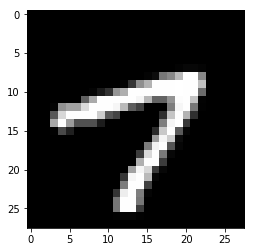
The Classic MNIST Dataset

The next examples will use the MNIST digits dataset. The previous examples used CSV files to load training data. Most neural network frameworks, such as Keras, have common training sets built in. This makes it easy to run the example, but hard to abstract the example to your own data. Your on data are not likely built into Keras. However, the MNIST data is complex enough that it is beyond the scope of this article to discuss how to load it. We will use the MNIST data build into Keras.

1
2
3
4
5
6
7
8
from keras.datasets import mnist
(x_train, y_train), (x_test, y_test) = mnist.load_data()

print("Shape of x_train: {}".format(x_train.shape))
print("Shape of y_train: {}".format(y_train.shape))
print()
print("Shape of x_test: {}".format(x_test.shape))
print("Shape of y_test: {}".format(y_test.shape))
1
2
3
4
5
Shape of x_train: (60000, 28, 28)
Shape of y_train: (60000,)

Shape of x_test: (10000, 28, 28)
Shape of y_test: (10000,)
1
2
3
4
5
6
7
8
9
10
# Display as image
%matplotlib inline
import matplotlib.pyplot as plt
import numpy as np

digit = 101 # Change to choose new digit

a = x_train[digit]
plt.imshow(a, cmap='gray', interpolation='nearest')
print("Image (#{}): Which is digit '{}'".format(digit,y_train[digit]))
1
Image (#101): Which is digit '7'

png

Convolutional Neural Networks

Convolutional Neural Networks are specifically for images. They have been applied to other cases; however, use beyond images is somewhat rarer than with images.

1
2
3
4
5
6
7
8
9
10
11
12
13
14
15
16
17
18
19
20
21
22
23
24
25
26
27
28
29
30
31
32
33
34
35
36
37
38
39
40
41
42
43
44
45
46
47
48
49
50
51
52
53
54
55
56
57
58
59
import keras
from keras.datasets import mnist
from keras.models import Sequential
from keras.layers import Dense, Dropout, Flatten
from keras.layers import Conv2D, MaxPooling2D
from keras import backend as K

batch_size = 128
num_classes = 10
epochs = 12

# input image dimensions
img_rows, img_cols = 28, 28

if K.image_data_format() == 'channels_first':
x_train = x_train.reshape(x_train.shape[0], 1, img_rows, img_cols)
x_test = x_test.reshape(x_test.shape[0], 1, img_rows, img_cols)
input_shape = (1, img_rows, img_cols)
else:
x_train = x_train.reshape(x_train.shape[0], img_rows, img_cols, 1)
x_test = x_test.reshape(x_test.shape[0], img_rows, img_cols, 1)
input_shape = (img_rows, img_cols, 1)

x_train = x_train.astype('float32')
x_test = x_test.astype('float32')
x_train /= 255
x_test /= 255
print('x_train shape:', x_train.shape)
print("Training samples: {}".format(x_train.shape[0]))
print("Test samples: {}".format(x_test.shape[0]))

# convert class vectors to binary class matrices
y_train = keras.utils.to_categorical(y_train, num_classes)
y_test = keras.utils.to_categorical(y_test, num_classes)

model = Sequential()
model.add(Conv2D(32, kernel_size=(3, 3),
activation='relu',
input_shape=input_shape))
model.add(Conv2D(64, (3, 3), activation='relu'))
model.add(MaxPooling2D(pool_size=(2, 2)))
model.add(Dropout(0.25))
model.add(Flatten())
model.add(Dense(128, activation='relu'))
model.add(Dropout(0.5))
model.add(Dense(num_classes, activation='softmax'))

model.compile(loss=keras.losses.categorical_crossentropy,
optimizer=keras.optimizers.Adadelta(),
metrics=['accuracy'])

model.fit(x_train, y_train,
batch_size=batch_size,
epochs=epochs,
verbose=2,
validation_data=(x_test, y_test))
score = model.evaluate(x_test, y_test, verbose=0)
print('Test loss: {}'.format(score[0]))
print('Test accuracy: {}'.format(score[1]))
1
2
3
4
5
6
7
8
9
10
11
12
13
14
15
16
17
18
19
20
21
22
23
24
25
26
27
28
29
30
x_train shape: (60000, 28, 28, 1)
Training samples: 60000
Test samples: 10000
Train on 60000 samples, validate on 10000 samples
Epoch 1/12
271s - loss: 0.3435 - acc: 0.8950 - val_loss: 0.0817 - val_acc: 0.9755
Epoch 2/12
269s - loss: 0.1171 - acc: 0.9660 - val_loss: 0.0581 - val_acc: 0.9813
Epoch 3/12
458s - loss: 0.0885 - acc: 0.9742 - val_loss: 0.0453 - val_acc: 0.9859
Epoch 4/12
554s - loss: 0.0743 - acc: 0.9778 - val_loss: 0.0382 - val_acc: 0.9867
Epoch 5/12
261s - loss: 0.0642 - acc: 0.9810 - val_loss: 0.0346 - val_acc: 0.9887
Epoch 6/12
321s - loss: 0.0594 - acc: 0.9826 - val_loss: 0.0337 - val_acc: 0.9888
Epoch 7/12
309s - loss: 0.0515 - acc: 0.9846 - val_loss: 0.0335 - val_acc: 0.9890
Epoch 8/12
317s - loss: 0.0477 - acc: 0.9857 - val_loss: 0.0337 - val_acc: 0.9890
Epoch 9/12
308s - loss: 0.0448 - acc: 0.9870 - val_loss: 0.0330 - val_acc: 0.9889
Epoch 10/12
322s - loss: 0.0416 - acc: 0.9873 - val_loss: 0.0307 - val_acc: 0.9901
Epoch 11/12
326s - loss: 0.0394 - acc: 0.9879 - val_loss: 0.0300 - val_acc: 0.9899
Epoch 12/12
313s - loss: 0.0367 - acc: 0.9887 - val_loss: 0.0313 - val_acc: 0.9902
Test loss: 0.03131893762472173
Test accuracy: 0.9902

Long Short Term Memory (LSTM)

Long Short Term Memory is typically used for either time series or natural language processing (which can be thought of as a special case of natural language processing).

1
2
3
4
5
6
7
8
9
10
11
12
13
14
15
16
17
18
19
20
21
22
23
24
25
26
27
28
29
30
31
32
33
34
35
36
37
38
39
40
from keras.preprocessing import sequence
from keras.models import Sequential
from keras.layers import Dense, Embedding
from keras.layers import LSTM
from keras.datasets import imdb
import numpy as np

max_features = 4 # 0,1,2,3 (total of 4)
x = [
[[0],[1],[1],[0],[0],[0]],
[[0],[0],[0],[2],[2],[0]],
[[0],[0],[0],[0],[3],[3]],
[[0],[2],[2],[0],[0],[0]],
[[0],[0],[3],[3],[0],[0]],
[[0],[0],[0],[0],[1],[1]]
]
x = np.array(x,dtype=np.float32)
y = np.array([1,2,3,2,3,1],dtype=np.int32)

# Convert y2 to dummy variables
y2 = np.zeros((y.shape[0], max_features),dtype=np.float32)
y2[np.arange(y.shape[0]), y] = 1.0
print(y2)

print('Build model...')
model = Sequential()
model.add(LSTM(128, dropout=0.2, recurrent_dropout=0.2, input_dim=1))
model.add(Dense(4, activation='sigmoid'))

# try using different optimizers and different optimizer configs
model.compile(loss='binary_crossentropy',
optimizer='adam',
metrics=['accuracy'])

print('Train...')
model.fit(x,y2,epochs=200)
pred = model.predict(x)
predict_classes = np.argmax(pred,axis=1)
print("Predicted classes: {}",predict_classes)
print("Expected classes: {}",predict_classes)
1
2
3
4
5
6
7
8
9
10
11
12
13
14
15
16
17
18
19
20
21
22
23
24
25
26
27
28
29
30
31
32
33
34
35
[[ 0.  1.  0.  0.]
[ 0. 0. 1. 0.]
[ 0. 0. 0. 1.]
[ 0. 0. 1. 0.]
[ 0. 0. 0. 1.]
[ 0. 1. 0. 0.]]
Build model...


c:\users\jeffh\anaconda3\envs\tf-latest\lib\site-packages\ipykernel\__main__.py:27: UserWarning: The `input_dim` and `input_length` arguments in recurrent layers are deprecated. Use `input_shape` instead.
c:\users\jeffh\anaconda3\envs\tf-latest\lib\site-packages\ipykernel\__main__.py:27: UserWarning: Update your `LSTM` call to the Keras 2 API: `LSTM(128, input_shape=(None, 1), recurrent_dropout=0.2, dropout=0.2)`


Train...
Epoch 1/200
6/6 [==============================] - 2s - loss: 0.7078 - acc: 0.5000
Epoch 2/200
6/6 [==============================] - 0s - loss: 0.7006 - acc: 0.5000
Epoch 3/200
6/6 [==============================] - 0s - loss: 0.6896 - acc: 0.6667
Epoch 4/200
6/6 [==============================] - 0s - loss: 0.6861 - acc: 0.6667
Epoch 5/200
6/6 [==============================] - 0s - loss: 0.6754 - acc: 0.7083

...

Epoch 198/200
6/6 [==============================] - 0s - loss: 0.2266 - acc: 0.9167
Epoch 199/200
6/6 [==============================] - 0s - loss: 0.2907 - acc: 0.8750
Epoch 200/200
6/6 [==============================] - 0s - loss: 0.1996 - acc: 0.9167
Predicted classes: {} [1 2 3 2 3 1]
Expected classes: {} [1 2 3 2 3 1]

Load/Save a Neural Network

It is very important to be able to load and save neural networks. This allows your neural network to be used each time without retraining.

1
2
3
4
5
6
7
8
9
10
11
12
13
14
15
16
17
18
19
20
21
22
23
import pandas as pd
import io
import requests
import numpy as np
from sklearn import metrics
from keras.models import Sequential
from keras.layers.core import Dense, Activation
from keras.models import load_model

url="https://raw.githubusercontent.com/jeffheaton/t81_558_deep_learning/master/data/auto-mpg.csv"
df=pd.read_csv(io.StringIO(requests.get(url).content.decode('utf-8')),na_values=['NA','?'])

cars = df['name']
df.drop('name',1,inplace=True)
missing_median(df, 'horsepower')
x,y = to_xy(df,"mpg")

model = Sequential()
model.add(Dense(10, input_dim=x.shape[1], kernel_initializer='normal', activation='relu'))
model.add(Dense(1, kernel_initializer='normal'))
model.compile(loss='mean_squared_error', optimizer='adam')

model.fit(x,y,verbose=2,epochs=100)
1
2
3
4
5
6
7
8
9
10
11
12
13
14
15
16
17
18
19
Epoch 1/100
0s - loss: 188.3123
Epoch 2/100
0s - loss: 180.3333
Epoch 3/100
0s - loss: 177.1118
Epoch 4/100
0s - loss: 173.3682
Epoch 5/100
0s - loss: 167.0144

...

Epoch 98/100
0s - loss: 11.2297
Epoch 99/100
0s - loss: 11.0280
Epoch 100/100
0s - loss: 10.9314
1
2
3
4
5
6
7
8
9
10
11
12
13
14
15
16
17
18
pred = model.predict(x)

# Measure RMSE error. RMSE is common for regression.
score = np.sqrt(metrics.mean_squared_error(pred,y))
print("Before save score (RMSE): {}".format(score))

# save neural network structure to JSON (no weights)
model_json = model.to_json()
with open("network.json", "w") as json_file:
json_file.write(model_json)

# save neural network structure to YAML (no weights)
model_yaml = model.to_yaml()
with open("network.yaml", "w") as yaml_file:
yaml_file.write(model_yaml)

# save entire network to HDF5 (save everything, suggested)
model.save("network.h5")
1
Before save score (RMSE): 3.276093006134033
1
2
3
4
5
6
7
from keras.models import load_model

model2 = load_model('network.h5')

# Measure RMSE error. RMSE is common for regression.
score = np.sqrt(metrics.mean_squared_error(pred,y))
print("After load score (RMSE): {}".format(score))
1
After load score (RMSE): 3.276093006134033